Data Structures and Algorithms

DSA Interview Questions

Kruskal’s Algorithm for Minimum Spanning Tree (MST)

Discover how Kruskal’s Algorithm constructs a Minimum Spanning Tree (MST) using a greedy strategy that ensures the lowest possible total weight. If you’re eager to enhance your algorithms expertise and receive free resources or stay updated on new courses, sign up here for our complimentary offerings and the latest updates tailored just for you.

Minimum Spanning Tree (MST)

A Minimum Spanning Tree (MST), also known as a minimum weight spanning tree, is a subset of the edges in a connected, undirected, and weighted graph that connects all vertices without forming any cycles and has the minimum possible total edge weight. In simple terms, it’s a tree that spans all the vertices of the graph while keeping the total weight as low as possible.

The weight of a spanning tree refers to the sum of the weights of all the edges included in that tree.

Understanding Kruskal’s Algorithm

Kruskal’s Algorithm is one of the most efficient methods to find the Minimum Spanning Tree in a graph. The algorithm follows a greedy approach, which means it builds the MST step by step by always choosing the lowest weight edge that does not form a cycle.

The process starts by sorting all edges in ascending order of weight. Then, it continues to add edges to the MST, one by one, as long as they do not result in a cycle. The algorithm prioritizes the edge with the smallest weight first and the largest weight last. This behavior of making the best local choice at each step helps in arriving at the globally optimal solution.

Because of this approach, Kruskal’s Algorithm is classified as a Greedy Algorithm.

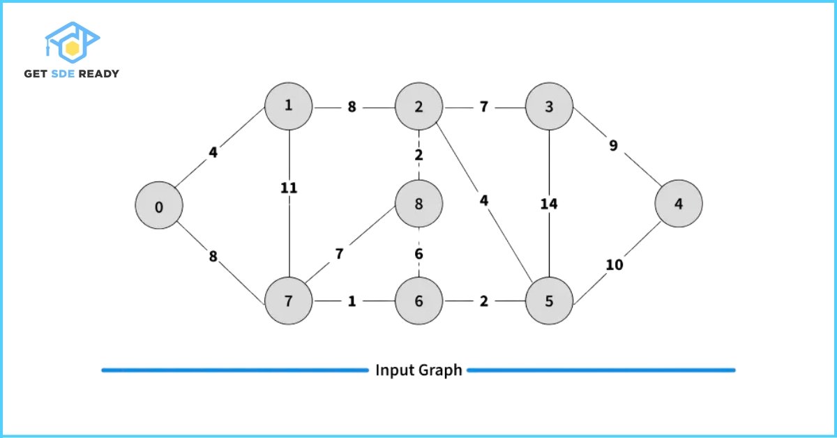
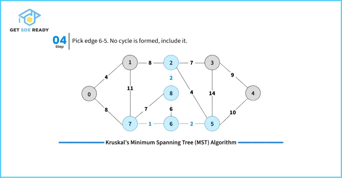
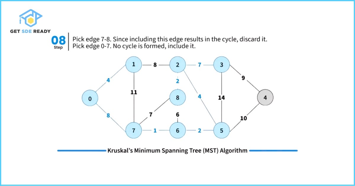
How to Find the MST Using Kruskal’s Algorithm?

To construct a Minimum Spanning Tree using Kruskal’s Algorithm, follow these steps:

Sort all edges in the graph in non-decreasing order based on their weights.
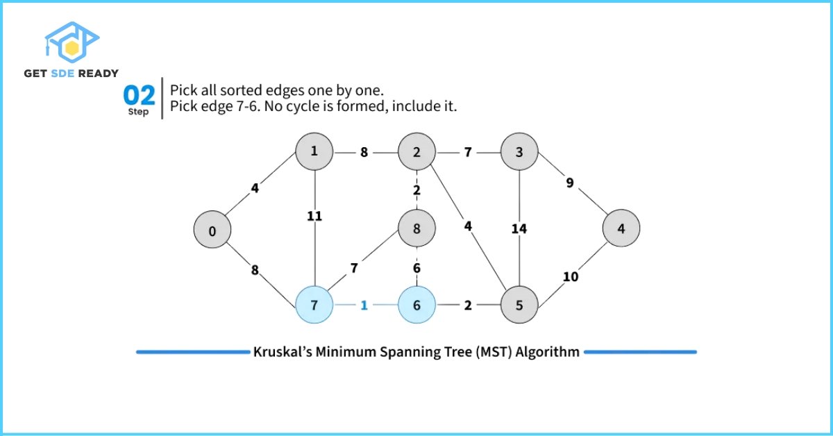
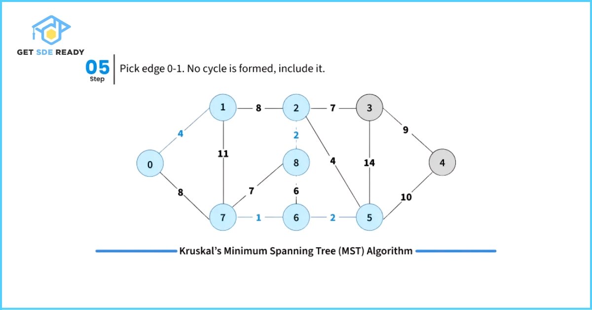
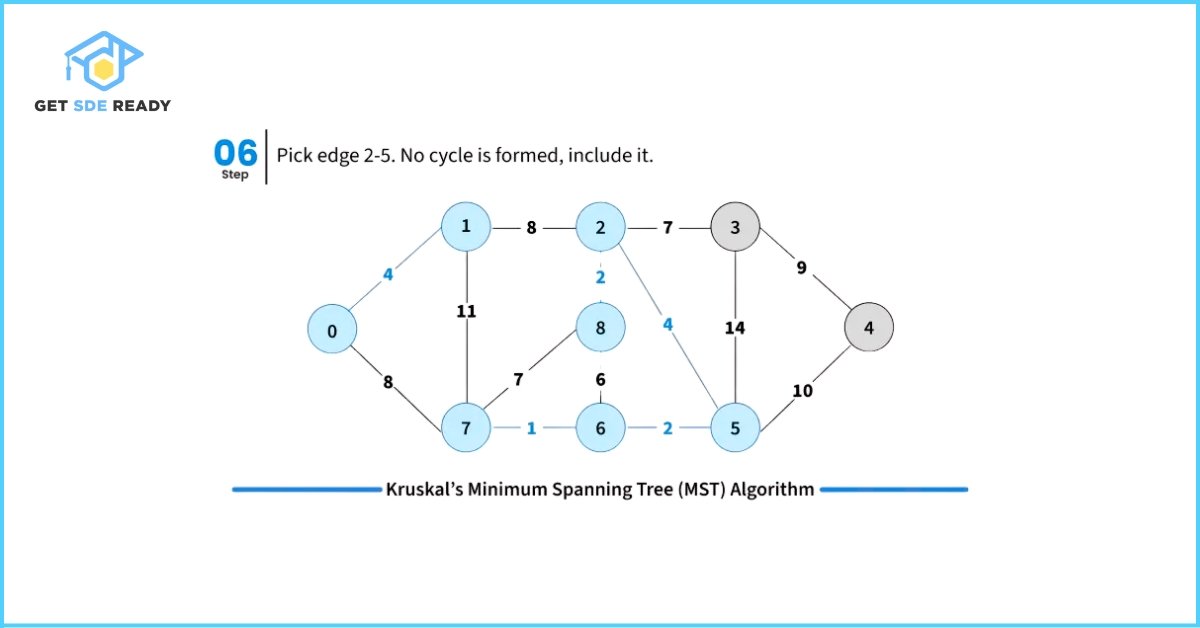
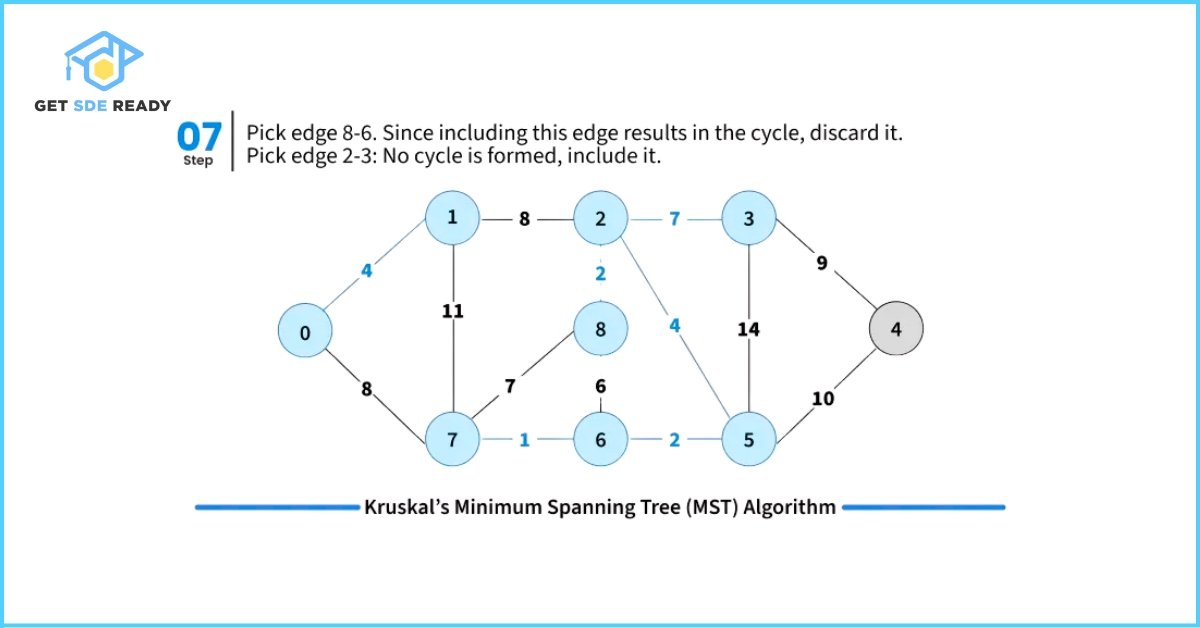
Pick the smallest weight edge. Check whether adding this edge creates a cycle in the spanning tree formed so far.
- If it does not form a cycle, include the edge in the MST.
- If it forms a cycle, discard the edge.
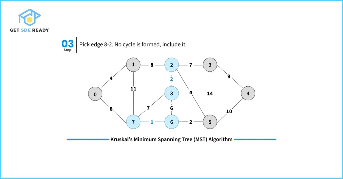
Repeat step 2 until the spanning tree contains exactly (V – 1) edges, where V is the number of vertices in the graph.

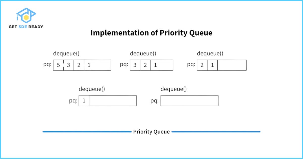
To efficiently check for cycles during this process, Kruskal’s Algorithm uses the Disjoint Set Data Structure (also known as Union-Find). This helps keep track of the connected components and efficiently determines whether including a new edge will cause a cycle.

Example of Descending order Priority Queue 2

Example of Descending order Priority Queue 1

				
					#include <bits/stdc++.h>
using namespace std;

// Disjoint set data struture
class DSU {
    vector<int> parent, rank;

public:
    DSU(int n) {
        parent.resize(n);
        rank.resize(n);
        for (int i = 0; i < n; i++) {
            parent[i] = i;
            rank[i] = 1;
        }
    }

    int find(int i) {
        return (parent[i] == i) ? i : (parent[i] = find(parent[i]));
    }

    void unite(int x, int y) {
        int s1 = find(x), s2 = find(y);
        if (s1 != s2) {
            if (rank[s1] < rank[s2]) parent[s1] = s2;
            else if (rank[s1] > rank[s2]) parent[s2] = s1;
            else parent[s2] = s1, rank[s1]++;
        }
    }
};
bool comparator(vector<int> &a,vector<int> &b){
    if(a[2]<=b[2])return true;
    return false;
}
int kruskalsMST(int V, vector<vector<int>> &edges) {
    
    // Sort all edhes
    sort(edges.begin(), edges.end(),comparator);
    
    // Traverse edges in sorted order
    DSU dsu(V);
    int cost = 0, count = 0;
    
    for (auto &e : edges) {
        int x = e[0], y = e[1], w = e[2];
        
        // Make sure that there is no cycle
        if (dsu.find(x) != dsu.find(y)) {
            dsu.unite(x, y);
            cost += w;
            if (++count == V - 1) break;
        }
    }
    return cost;
}

int main() {
    
    // An edge contains, weight, source and destination
    vector<vector<int>> edges = {
        {0, 1, 10}, {1, 3, 15}, {2, 3, 4}, {2, 0, 6}, {0, 3, 5}
    };
    
    cout<<kruskalsMST(4, edges);
    
    return 0;
}

Searching

Traverse the loop to find a target value, requiring safeguards against infinite loops.

For a quick refresher on these operations, try our crash course.

Implementation of Circular Linked Lists

Let’s see how circular linked lists come to life in code. Below are examples in C, C++, and Java for inserting nodes at the beginning and end.

				
					import java.util.Arrays;
import java.util.Comparator;

class GfG {
    public static int kruskalsMST(int V, int[][] edges) {
        
        // Sort all edges based on weight
        Arrays.sort(edges, Comparator.comparingInt(e -> e[2]));
        
        // Traverse edges in sorted order
        DSU dsu = new DSU(V);
        int cost = 0, count = 0;
        
        for (int[] e : edges) {
            int x = e[0], y = e[1], w = e[2];
            
            // Make sure that there is no cycle
            if (dsu.find(x) != dsu.find(y)) {
                dsu.union(x, y);
                cost += w;
                if (++count == V - 1) break;
            }
        }
        return cost;
    }

    public static void main(String[] args) {
        
        // An edge contains, weight, source and destination
        int[][] edges = {
            {0, 1, 10}, {1, 3, 15}, {2, 3, 4}, {2, 0, 6}, {0, 3, 5}
        };
        
       System.out.println(kruskalsMST(4, edges));
    }
}

// Disjoint set data structure
class DSU {
    private int[] parent, rank;

    public DSU(int n) {
        parent = new int[n];
        rank = new int[n];
        for (int i = 0; i < n; i++) {
            parent[i] = i;
            rank[i] = 1;
        }
    }

    public int find(int i) {
        if (parent[i] != i) {
            parent[i] = find(parent[i]);
        }
        return parent[i];
    }

    public void union(int x, int y) {
        int s1 = find(x);
        int s2 = find(y);
        if (s1 != s2) {
            if (rank[s1] < rank[s2]) {
                parent[s1] = s2;
            } else if (rank[s1] > rank[s2]) {
                parent[s2] = s1;
            } else {
                parent[s2] = s1;
                rank[s1]++;
            }
        }
    }
}

				
					function kruskalsMST(V, edges) {
    
    // Sort all edges
    edges.sort((a, b) => a[2] - b[2]);
    
    // Traverse edges in sorted order
    const dsu = new DSU(V);
    let cost = 0;
    let count = 0;
    for (const [x, y, w] of edges) {
        
        // Make sure that there is no cycle
        if (dsu.find(x) !== dsu.find(y)) {
            dsu.unite(x, y);
            cost += w;
            if (++count === V - 1) break;
        }
    }
    return cost;
}

// Disjoint set data structure
class DSU {
    constructor(n) {
        this.parent = Array.from({ length: n }, (_, i) => i);
        this.rank = Array(n).fill(1);
    }

    find(i) {
        if (this.parent[i] !== i) {
            this.parent[i] = this.find(this.parent[i]);
        }
        return this.parent[i];
    }

    unite(x, y) {
        const s1 = this.find(x);
        const s2 = this.find(y);
        if (s1 !== s2) {
            if (this.rank[s1] < this.rank[s2]) this.parent[s1] = s2;
            else if (this.rank[s1] > this.rank[s2]) this.parent[s2] = s1;
            else {
                this.parent[s2] = s1;
                this.rank[s1]++;
            }
        }
    }
}

const edges = [
    [0, 1, 10], [1, 3, 15], [2, 3, 4], [2, 0, 6], [0, 3, 5]
];
console.log(kruskalsMST(4, edges));

				
					from functools import cmp_to_key

def comparator(a,b):
    return a[2] - b[2];

def kruskals_mst(V, edges):

    # Sort all edges
    edges = sorted(edges,key=cmp_to_key(comparator))
    
    # Traverse edges in sorted order
    dsu = DSU(V)
    cost = 0
    count = 0
    for x, y, w in edges:
        
        # Make sure that there is no cycle
        if dsu.find(x) != dsu.find(y):
            dsu.union(x, y)
            cost += w
            count += 1
            if count == V - 1:
                break
    return cost
    
# Disjoint set data structure
class DSU:
    def __init__(self, n):
        self.parent = list(range(n))
        self.rank = [1] * n

    def find(self, i):
        if self.parent[i] != i:
            self.parent[i] = self.find(self.parent[i])
        return self.parent[i]

    def union(self, x, y):
        s1 = self.find(x)
        s2 = self.find(y)
        if s1 != s2:
            if self.rank[s1] < self.rank[s2]:
                self.parent[s1] = s2
            elif self.rank[s1] > self.rank[s2]:
                self.parent[s2] = s1
            else:
                self.parent[s2] = s1
                self.rank[s1] += 1


if __name__ == '__main__':
    
    # An edge contains, weight, source and destination
    edges = [[0, 1, 10], [1, 3, 15], [2, 3, 4], [2, 0, 6], [0, 3, 5]]
    print(kruskals_mst(4, edges))

Output: Shortest Path Distance Matrix

  4   5   5   7
  0   1   4   6
  6   0   3   5
  7   1   0   2
  5   5   4   0

Each number represents the shortest distance from the row node to the column node after applying the Floyd-Warshall algorithm.

Time Complexity

The algorithm runs in O(V³) time, where V is the number of vertices. This complexity arises from three nested loops, each iterating over all vertices.

Auxiliary Space

The space complexity is O(1) beyond the input distance matrix, as the algorithm updates the matrix in place without requiring additional significant storage.

Note

The above implementation of the Floyd-Warshall algorithm only computes and prints the shortest distances between all pairs of nodes.

If you want to also reconstruct and print the actual shortest paths, the algorithm can be modified by maintaining a predecessor matrix (or parent matrix). This separate 2D matrix stores the predecessor of each node on the shortest path, allowing you to trace back the path from the destination node to the source node.

Real-World Applications of the Floyd-Warshall Algorithm

1. Network Routing in Computer Networking

The Floyd-Warshall algorithm is widely used in computer networks to determine the shortest paths between all pairs of nodes. This helps in efficient routing of data packets, ensuring optimal communication paths in network infrastructure.

2. Flight Connectivity in Aviation

In the aviation industry, this algorithm assists in finding the shortest and most cost-effective routes between airports, optimizing flight paths and connections for passengers and cargo.

3. Geographic Information Systems (GIS)

GIS applications frequently analyze spatial data such as road networks. Floyd-Warshall is used to calculate the shortest paths between various locations, helping in navigation, urban planning, and resource management.

4. Kleene’s Algorithm and Formal Language Theory

A generalization of Floyd-Warshall, known as Kleene’s algorithm, is employed in automata theory to compute regular expressions for regular languages, facilitating pattern matching and compiler design.

Network Routing in Computer Networking

Flight Connectivity in Aviation

In the aviation industry, this algorithm assists in finding the shortest and most cost-effective routes between airports, optimizing flight paths and connections for passengers and cargo.

Geographic Information Systems (GIS)

Kleene’s Algorithm and Formal Language Theory

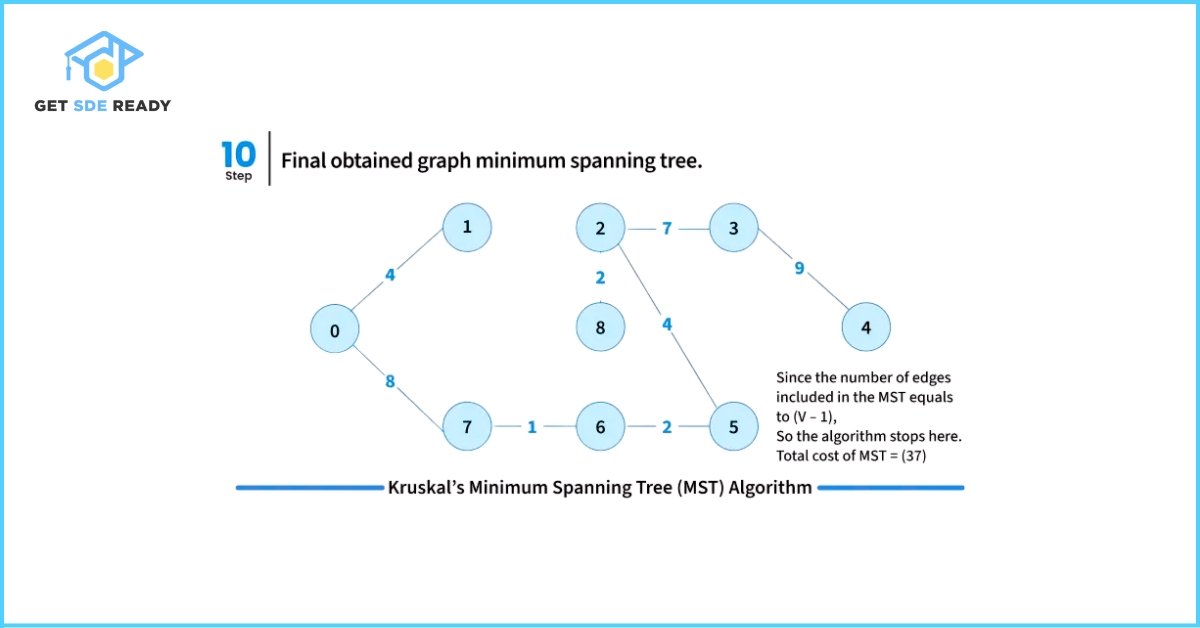
Output

Below are the edges included in the constructed Minimum Spanning Tree (MST):

Edge: 2 — 3 | Weight: 4

Edge: 0 — 3 | Weight: 5

Edge: 0 — 1 | Weight: 10

Total Weight of the Minimum Spanning Tree: 19

Time and Space Complexity of Kruskal’s Algorithm

Time Complexity

O(E * log E) or O(E * log V)

The most time-consuming step in Kruskal’s Algorithm is sorting all the edges by their weight. If there are E edges, sorting them requires O(E * log E) time.

Once the edges are sorted, the algorithm processes each edge and uses the Disjoint Set Union-Find structure to check for cycles. The find and union operations can be performed in O(log V) time using path compression and union by rank.

Therefore, the total time complexity becomes:

O(E * log E) + O(E * log V) = O(E * log E + E * log V)

Since the number of edges E can be as large as O(V²) in a dense graph, both log V and log E grow similarly. Hence, the time complexity is often simplified to:

O(E * log E) or O(E * log V)

Auxiliary Space Complexity:

O(E + V)

The algorithm requires extra space to store the disjoint set (Union-Find) data structure and the sorted list of edges. As a result, the auxiliary space used is proportional to the number of vertices and edges, i.e., O(V + E).

What is the main difference between Kruskal’s and Prim’s algorithms?

Kruskal’s algorithm is edge-centric, sorting all edges first and picking the smallest one that doesn’t form a cycle; Prim’s is vertex-centric, growing a tree from a starting vertex by adding the smallest edge connecting to the tree. If you prefer structured, step-by-step guidance on spanning tree algorithms, check out our DSA Course for expert-led tutorials.

How does Union-Find (DSU) speed up cycle detection in Kruskal’s Algorithm?

By keeping track of connected components in a tree-like structure. Each find operation locates the root parent of a vertex (compressing paths along the way), and union merges two components by rank. This nearly constant-time check avoids expensive cycle detection via traversal. If you want to see DSU and other algorithmic fundamentals applied in web-based projects, explore our Web Development Course.

Can Kruskal’s Algorithm handle graphs with negative edge weights?

Yes—since Kruskal’s sorts edges by weight, it will include negative-weight edges first (if they don’t create a cycle). The algorithm still produces the MST correctly, even if some edge weights are negative. For comprehensive practice problems on graph algorithms, consider enrolling in our Design DSA Combined program.

DSA, High & Low Level System Designs

85+ Live Classes & Recordings
24*7 Live Doubt Support
400+ DSA Practice Questions
Comprehensive Notes
HackerRank Tests & Quizzes
Topic-wise Quizzes
Case Studies
Access to Global Peer Community

Buy for 60% OFF
₹25,000.00 ₹9,999.00

Accelerate your Path to a Product based Career

Boost your career or get hired at top product-based companies by joining our expertly crafted courses. Gain practical skills and real-world knowledge to help you succeed.

Reach Out Now

If you have any queries, please fill out this form. We will surely reach out to you.

Contact Email

Reach us at the following email address.

[email protected]

Phone Number

You can reach us by phone as well.

+91-97737 28034

Our Location

Rohini, Sector-3, Delhi-110085

Kruskal’s Algorithm for Minimum Spanning Tree (MST)

Minimum Spanning Tree (MST)

Understanding Kruskal’s Algorithm

How to Find the MST Using Kruskal’s Algorithm?

Searching

Implementation of Circular Linked Lists

Output: Shortest Path Distance Matrix

Time Complexity

Auxiliary Space

Note

Real-World Applications of the Floyd-Warshall Algorithm

1. Network Routing in Computer Networking

2. Flight Connectivity in Aviation

3. Geographic Information Systems (GIS)

4. Kleene’s Algorithm and Formal Language Theory

Network Routing in Computer Networking

Flight Connectivity in Aviation

Geographic Information Systems (GIS)

Kleene’s Algorithm and Formal Language Theory

Output

Time and Space Complexity of Kruskal’s Algorithm

Time Complexity

Auxiliary Space Complexity:

What is the main difference between Kruskal’s and Prim’s algorithms?

How does Union-Find (DSU) speed up cycle detection in Kruskal’s Algorithm?

Can Kruskal’s Algorithm handle graphs with negative edge weights?

DSA, High & Low Level System Designs

Buy for 60% OFF ₹25,000.00 ₹9,999.00

Accelerate your Path to a Product based Career

Design Patterns Bootcamp

Buy for 50% OFF ₹2,000.00 ₹999.00

LLD Bootcamp

Buy for 50% OFF ₹2,000.00 ₹999.00

Essentials of Machine Learning and Artificial Intelligence

Buy for 65% OFF ₹20,000.00 ₹6,999.00

Fast-Track to Full Spectrum Software Engineering

Buy for 57% OFF ₹35,000.00 ₹14,999.00

DSA, High & Low Level System Designs

Buy for 60% OFF ₹25,000.00 ₹9,999.00

Low & High Level System Design

Buy for 65% OFF ₹20,000.00 ₹6,999.00

Reach Out Now

Contact Email

Phone Number

Our Location

Quick Links

Quick Links

Social Media

Master Your Interviews with Our Free Roadmap!

Hi Instagram Fam! Get a FREE Cheat Sheet on System Design.

Hi LinkedIn Fam! Get a FREE Cheat Sheet on System Design

Loved Our YouTube Videos? Get a FREE Cheat Sheet on System Design.

Buy for 60% OFF
₹25,000.00 ₹9,999.00

Buy for 50% OFF
₹2,000.00 ₹999.00

Buy for 50% OFF
₹2,000.00 ₹999.00

Buy for 65% OFF
₹20,000.00 ₹6,999.00

Buy for 57% OFF
₹35,000.00 ₹14,999.00

Buy for 60% OFF
₹25,000.00 ₹9,999.00

Buy for 65% OFF
₹20,000.00 ₹6,999.00

Hi Instagram Fam!
Get a FREE Cheat Sheet on System Design.

Hi LinkedIn Fam!
Get a FREE Cheat Sheet on System Design