Conditional Formatting
Conditional Formatting is a powerful Excel feature that allows users to visually highlight specific data points, trends, or anomalies within a spreadsheet based on defined rules. It enhances data interpretation by automatically changing the appearance of cells—such as their color, font, or border—based on the content they contain.
What is Conditional Formatting?
Conditional Formatting applies custom formatting to cells when certain criteria are met. It transforms raw numbers into visual cues, making it easier to:
- Detect patterns.
- Identify high or low values.
- Spot duplicates or errors.
- Compare results against thresholds.
Common Conditional Formatting Options
- Highlight Cell Rules: Formats cells based on value comparisons (e.g., greater than, less than, equal to).
- Top/Bottom Rules: Highlights top 10 items, top 10%, or below average values.
- Data Bars: Adds a horizontal bar inside the cell to show relative value.
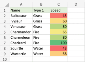
- Color Scales: Applies gradient colors to represent value ranges.
- Icon Sets: Displays symbols like arrows, flags, or traffic lights to indicate data status.
How It Helps in Data Analysis
- Performance Review: Highlight underperforming products or employees.
- Financial Analysis: Mark profit margins below a threshold.
- Trend Tracking: Use color scales to view monthly growth or decline.
- Quality Control: Instantly spot values outside an acceptable range.
Practical Scenarios
- In a sales sheet, you can use Conditional Formatting to turn high sales green and low sales red.
- For student marks, apply formatting to highlight scores below the passing grade.
- In inventory management, use icon sets to indicate stock levels: full, moderate, or low.
Best Practices
- Don’t overuse: Too many colors can overwhelm users.
- Combine with filters and sorting for deeper insights.
- Keep the formatting consistent and meaningful to support decision-making.
