Hashing: Static and Dynamic Hashing
Hashing is a fast and direct way to access data using a key. Instead of searching through data sequentially, a hash function converts the key into a hash value (bucket address) where the actual data is stored. It is widely used in indexing, especially when quick access based on equality conditions is needed (e.g., searching by ID).
Static Hashing
In static hashing, the number of primary buckets is fixed when the hash table is created and doesn’t change over time.
For example, if we have a data record for employee_id = 107, the hash function is mod-5 which is – H(x) % 5, where x = id. Then the operation will take place like this:
H(106) % 5 = 1.
This indicates that the data record should be placed or searched in the 1st bucket (or 1st hash index) in the hash table.
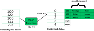
The primary key is used as the input to the hash function and the hash function generates the output as the hash index (bucket's address) which contains the address of the actual data record on the disk block.

How It Works:
- A hash function (e.g.,
h(k) = k mod M) maps a keykto one of theMbuckets. - Buckets are stored in memory or on disk.
- If multiple keys hash to the same bucket (a collision), it is handled using techniques like:
- Chaining (linked lists in the same bucket)
- Open addressing (probing nearby buckets)
Pros:
- Simple to implement
- Fast access for fixed-sized datasets
Cons:
- Suffers from overflow when too many keys map to the same bucket
- Not suitable for databases with growing or shrinking data sizes
- Wastes space or causes collisions if
Mis not well-chosen
Dynamic Hashing
Dynamic hashing allows the number of buckets to grow or shrink dynamically as data size changes. This solves the overflow and space waste problems of static hashing.
Example: If global depth: k = 2, the keys will be mapped accordingly to the hash index. K bits starting from LSB will be taken to map a key to the buckets. That leaves us with the following 4 possibilities: 00, 11, 10, 01.
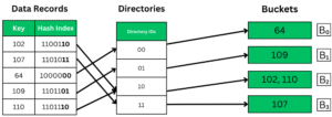
As we can see in the above image, the k bits from LSBs are taken in the hash index to map to their appropriate buckets through directory IDs. The hash indices point to the directories, and the k bits are taken from the directories’ IDs and then mapped to the buckets. Each bucket holds the value corresponding to the IDs converted in binary.
Common Method: Extendible Hashing
- Uses a directory that can grow in size.
- Hash function generates a binary string; only a prefix of bits is used to index the directory.
- Buckets split when they overflow, and the directory expands by adding more bits from the hash.
Example Process:
- Hash function outputs
h(k) = 101011... - If directory uses first 2 bits:
10→ Bucket 10 - If Bucket 10 overflows → Split it and use 3 bits now for this region
- Directory expands accordingly
Pros:
- Efficient for databases with changing size
- Reduces overflow handling complexity
- Keeps search time almost constant
Cons:
- Slightly more complex to implement
- Requires maintaining an extra directory
Comparison Table
| Feature | Static Hashing | Dynamic Hashing |
|---|---|---|
| Bucket Count | Fixed | Grows/shrinks as needed |
| Overflow Handling | Required (chaining/probing) | Rare (handled via bucket splits) |
| Space Efficiency | Lower (fixed buckets) | Higher (adjusts to data size) |
| Implementation | Simple | More complex |
| Performance on Growth | Degrades | Remains efficient |
When to Use
Static Hashing: Good for small or read-heavy datasets with a known fixed size.
Dynamic Hashing: Ideal for large, frequently changing databases where insertion and deletion are common.
