Data Structures and Algorithms

DSA Interview Questions

Graph Data Structure: Basics and Representations

Graphs power everything from social networks to route planning. If you’re ready to master graph algorithms and stay in the loop on new learning opportunities, sign up for free courses and get the latest updates today!

What is a Graph Data Structure?

A graph is a mathematical and computational model that represents a set of objects (called vertices) and the connections between them (called edges). These vertices and edges together form a network or structure, commonly represented as G(V, E), where V is the set of vertices and E is the set of edges.

Think of a football match: each player acts as a node, and their passes, movements, or interactions act as the edges connecting them. This web of activity mirrors a graph, and analyzing it can provide valuable insights into player roles, team cohesion, and strategic execution.

Components of a Graph Data Structure

1. Vertices (Nodes):

Vertices are the primary elements in a graph. They represent entities such as people in a network or players on a team. Vertices may carry data, and they can either be labeled (e.g., Player A, Player B) or unlabeled, depending on the use case.

find the fastest route mirrors graph traversal algorithms you’ll practice in our DSA Course.

2. Edges (Connections):

Edges define the relationships or links between vertices. In directed graphs, edges follow a specific direction (like a pass from Player A to Player B), while in undirected graphs, the connections are mutual. Edges can also be labeled or unlabelled and may represent various forms of interaction depending on the scenario. Sometimes, edges are also referred to as arcs.

Types of Graphs in Data Structures and Algorithms

Understanding the different types of graphs is essential for solving various real-world problems using data structures and algorithms. Below are the major types of graphs commonly encountered:

1. Null Graph

A null graph is the most basic form of a graph where no edges exist between the vertices. It represents a completely disconnected structure.

2. Trivial Graph

A trivial graph contains only a single vertex and no edges. It is considered the smallest possible graph.

3. Undirected Graph

In an undirected graph, the edges have no direction, meaning the relationship between vertices is mutual. Each edge simply connects two vertices without implying a one-way connection.

4. Directed Graph (Digraph)

A directed graph, or digraph, consists of edges that have a specific direction. Here, each edge is an ordered pair, representing a one-way connection from one vertex to another.

5. Connected Graph

A graph is called connected when there is a path between every pair of vertices. In other words, no node is isolated, and all vertices are reachable from any starting point.

6. Disconnected Graph

A disconnected graph has at least one vertex that is not reachable from another vertex. It consists of two or more disjoint subgraphs.

7. Regular Graph

A regular graph is one in which each vertex has the same number of connections. If every vertex has exactly K edges, the graph is called a K-regular graph.

8. Complete Graph

A complete graph is a type where each vertex is connected to every other vertex. For a graph with n vertices, it contains n(n-1)/2 edges in the undirected case.

9. Cycle Graph

A cycle graph forms a closed loop, where each vertex connects to exactly two other vertices. The graph forms a single continuous cycle.

10. Cyclic Graph

A cyclic graph contains at least one cycle, meaning a path exists in which the starting and ending vertex is the same.

11. Directed Acyclic Graph (DAG)

A Directed Acyclic Graph, or DAG, is a directed graph with no cycles. DAGs are especially useful in applications like task scheduling and dependency resolution.

12. Bipartite Graph

A bipartite graph is one where the vertex set can be divided into two distinct groups, and no two vertices within the same group are connected. Edges only connect vertices from one set to the other.

13. Weighted Graph

In a weighted graph, each edge carries an associated weight or cost. These weights can represent distance, time, or any quantifiable metric. Weighted graphs can be either directed or undirected.

Learn how these structures underpin modern system design in our Master DSA, Web-Dev & System Design program.

Representation of Graph Data Structure

Graphs can be stored in various ways depending on the requirements of space and time complexity. The two most widely used methods for representing graphs are:

Adjacency Matrix
Adjacency List

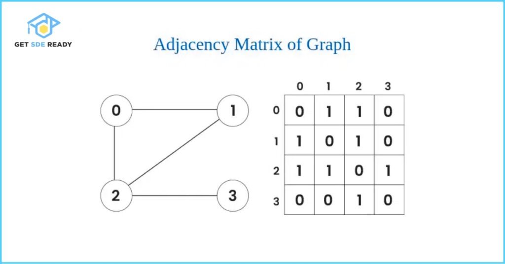
Adjacency Matrix Representation

In the adjacency matrix approach, a graph is represented using a two-dimensional array (or matrix). Each row and column in the matrix corresponds to a vertex in the graph. The value at a specific cell (i, j) indicates the presence and weight of an edge between vertex i and vertex j.

If the edge exists, the cell contains a non-zero value (usually the edge’s weight).
If there is no edge, the cell contains zero (or ∞ for weighted graphs without a direct connection).

This representation is particularly useful for dense graphs, where the number of edges is close to the number of vertex pairs.

Code Example: Adjacency Matrix Implementation

Here’s a basic implementation of a graph using an adjacency matrix:

				
					#include <iostream>
#include <vector>
using namespace std;

// Function to add an edge between two vertices
void addEdge(vector<vector<int>>& adj, int i, int j) {
    adj[i].push_back(j);
    adj[j].push_back(i); // Undirected
}

// Function to display the adjacency list
void displayAdjList(const vector<vector<int>>& adj) {
    for (int i = 0; i < adj.size(); i++) {
        cout << i << ": "; // Print the vertex
        for (int j : adj[i]) {
            cout << j << " "; // Print its adjacent
        }
        cout << endl; 
    }
}

// Main function
int main() {
    // Create a graph with 4 vertices and no edges
    int V = 4;
    vector<vector<int>> adj(V); 

    // Now add edges one by one
    addEdge(adj, 0, 1);
    addEdge(adj, 0, 2);
    addEdge(adj, 1, 2);
    addEdge(adj, 2, 3);

    cout << "Adjacency List Representation:" << endl;
    displayAdjList(adj);

    return 0;
}

Searching

Traverse the loop to find a target value, requiring safeguards against infinite loops.

For a quick refresher on these operations, try our crash course.

Implementation of Circular Linked Lists

Let’s see how circular linked lists come to life in code. Below are examples in C, C++, and Java for inserting nodes at the beginning and end.

				
					import java.util.ArrayList;
import java.util.List;

public class GfG {
    
    // Method to add an edge between two vertices
    public static void addEdge(List<List<Integer>> adj, int i, int j) {
        adj.get(i).add(j);
        adj.get(j).add(i); // Undirected
    }

    // Method to display the adjacency list
    public static void displayAdjList(List<List<Integer>> adj) {
        for (int i = 0; i < adj.size(); i++) {
            System.out.print(i + ": "); // Print the vertex
            for (int j : adj.get(i)) {
                System.out.print(j + " "); // Print its adjacent 
            }
            System.out.println(); 
        }
    }

    // Main method
    public static void main(String[] args) {
      
        // Create a graph with 4 vertices and no edges
        int V = 4;
        List<List<Integer>> adj = new ArrayList<>(V); 
        for (int i = 0; i < V; i++) {
            adj.add(new ArrayList<>());
        }

        // Now add edges one by one
        addEdge(adj, 0, 1);
        addEdge(adj, 0, 2);
        addEdge(adj, 1, 2);
        addEdge(adj, 2, 3);

        System.out.println("Adjacency List Representation:");
        displayAdjList(adj);
    }
}

				
					function addEdge(adj, i, j) {
    adj[i].push(j);
    adj[j].push(i); // Undirected
}

function displayAdjList(adj) {
    for (let i = 0; i < adj.length; i++) {
        console.log(`${i}: `); 
        for (const j of adj[i]) {
             console.log(`${j} `); 
        }
        console.log(); 
    }
}

// Create a graph with 4 vertices and no edges
const V = 4;
const adj = Array.from({ length: V }, () => []);

// Now add edges one by one
addEdge(adj, 0, 1);
addEdge(adj, 0, 2);
addEdge(adj, 1, 2);
addEdge(adj, 2, 3);

console.log("Adjacency List Representation:");
displayAdjList(adj);

				
					def add_edge(adj, i, j):
    adj[i].append(j)
    adj[j].append(i)  # Undirected

def display_adj_list(adj):
    for i in range(len(adj)):
        print(f"{i}: ", end="")
        for j in adj[i]:
            print(j, end=" ")
        print()

# Create a graph with 4 vertices and no edges
V = 4
adj = [[] for _ in range(V)]

# Now add edges one by one
add_edge(adj, 0, 1)
add_edge(adj, 0, 2)
add_edge(adj, 1, 2)
add_edge(adj, 2, 3)

print("Adjacency List Representation:")
display_adj_list(adj)

Output: Adjacency Matrix Representation

The following is the output of the adjacency matrix implementation shown above:

0 1 1 0

1 0 1 0

1 1 0 1

0 0 1 0

Each row of the matrix represents the connections of a specific vertex with all other vertices. For example:

The first row 0 1 1 0 shows that Vertex 0 is connected to Vertex 1 and Vertex 2.
The third row 1 1 0 1 indicates that Vertex 2 is connected to Vertex 0, 1, and 3.

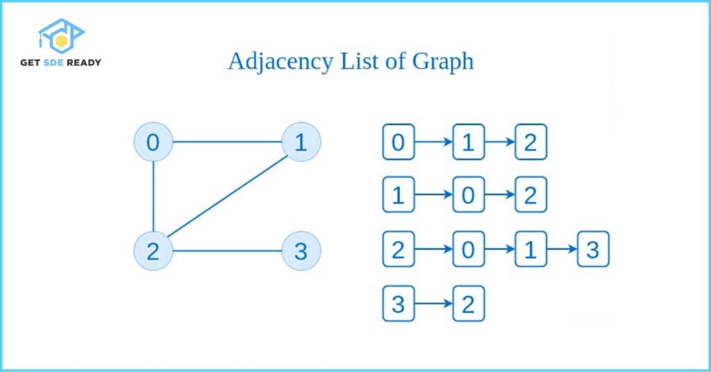
Adjacency List Representation of Graph

In the adjacency list method, a graph is represented using a list of lists (or a dictionary of lists). Each vertex has a corresponding list that stores all the vertices it is directly connected to. This approach is especially efficient for sparse graphs, where the number of edges is significantly less than the square of the number of vertices.

Think of it as an array (or dictionary) where each element represents a vertex, and it points to a list containing all its neighboring vertices.

This structure is memory-efficient and offers better performance when dealing with large graphs with fewer connections.

Code Example: Adjacency List Implementation

Here’s a simple Python implementation of a graph using an adjacency list:

				
					#include <iostream>
#include <vector>
using namespace std;

// Function to add an edge between two vertices
void addEdge(vector<vector<int>>& adj, int i, int j) {
    adj[i].push_back(j);
    adj[j].push_back(i); // Undirected
}

// Function to display the adjacency list
void displayAdjList(const vector<vector<int>>& adj) {
    for (int i = 0; i < adj.size(); i++) {
        cout << i << ": "; // Print the vertex
        for (int j : adj[i]) {
            cout << j << " "; // Print its adjacent
        }
        cout << endl; 
    }
}

// Main function
int main() {
    // Create a graph with 4 vertices and no edges
    int V = 4;
    vector<vector<int>> adj(V); 

    // Now add edges one by one
    addEdge(adj, 0, 1);
    addEdge(adj, 0, 2);
    addEdge(adj, 1, 2);
    addEdge(adj, 2, 3);

    cout << "Adjacency List Representation:" << endl;
    displayAdjList(adj);

    return 0;
}

Output: Adjacency List Representation

0: 1 2

1: 0 2

2: 0 1 3

3: 2

This output shows:

Vertex 0 is connected to vertices 1 and 2
Vertex 2 connects to 0, 1, and 3

Each line clearly represents the list of neighbors for a given vertex, making this format highly intuitive and easy to traverse when performing graph algorithms like BFS or DFS.

Comparison: Adjacency Matrix vs Adjacency List

Choosing the right representation for a graph depends on the nature of the graph—whether it’s sparse or dense—and the operations you intend to perform on it.

If the graph has a large number of edges (dense graph), the adjacency matrix is generally preferred. It allows constant-time access to check if an edge exists between two vertices.
For sparse graphs, where most pairs of vertices are not connected, an adjacency list is more efficient in terms of memory usage.

Algorithms like Prim’s and Dijkstra’s can benefit from the adjacency matrix due to its faster edge access times in dense graphs.

Performance Comparison Table

Operation	Adjacency Matrix	Adjacency List
Add Edge	O(1)	O(1)
Remove Edge	O(1)	O(N)
Initialization	O(N²)	O(N)

Add Edge: Both representations allow constant time addition of an edge.
Remove Edge: Removing an edge is faster in a matrix but slower in a list due to the need to search and delete.
Initialization: Matrix requires O(N²) space, while the list uses only O(N), making it more space-efficient for large graphs with fewer connections.

For a deeper dive into storage choices and trade-offs, check out our Essential DSA & Web-Dev Courses for Programmers.

Basic Operations on Graph Data Structure

Graphs support several fundamental operations essential for manipulating and analyzing their structure. These basic operations include:

Insertion and Deletion of Nodes (Vertices)
- Adding and Removing Vertices in both Adjacency List and Adjacency Matrix representations.
- In adjacency lists, vertices are added by creating new lists or entries, while in adjacency matrices, adding a vertex involves expanding the matrix size.
Insertion and Deletion of Edges
- Adding and Removing Edges in the Adjacency List involves updating the lists for the connected vertices.
- In the Adjacency Matrix, edges are represented by updating the corresponding cells in the matrix.
Searching in Graphs
- Searching refers to locating a specific node or edge within the graph. Efficient search algorithms depend on the graph’s representation.
Traversal of Graph
- Traversal means visiting all vertices (and edges) of the graph systematically. Common traversal techniques include Depth-First Search (DFS) and Breadth-First Search (BFS).

These operations form the backbone of graph algorithms and are critical for applications ranging from social network analysis to route optimization and beyond.

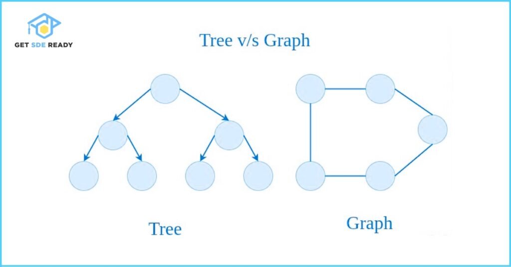
Difference Between Tree and Graph

A tree is a specialized form of a graph with additional constraints. While every tree qualifies as a graph, not every graph is a tree. Data structures such as linked lists, trees, and heaps can all be considered special cases of graphs with unique rules applied.

Real-Life Applications of Graph Data Structure

The Graph Data Structure plays a vital role in solving complex problems across many real-world domains. Here are some notable applications:

Unlike earlier studied data structures like arrays, linked lists, and trees—which have strict structural constraints (linear or hierarchical with no loops)—graphs allow random and flexible connections between nodes. This flexibility makes graphs ideal for modeling complex relationships found in real-world scenarios.
Social Networks: Each user is represented as a vertex (node), and edges represent connections like friendships or followers. Features such as mutual friends and network recommendations are naturally modeled as graph problems.
Computer Networks: Graphs effectively represent network topology, illustrating how routers, switches, and devices interconnect.
Transportation Networks: Graphs map connections between locations such as roads, airports, and transit routes, facilitating route optimization and planning.
Neural Networks: Here, vertices symbolize neurons, and edges represent synapses. Neural networks help understand brain function and learning by modeling approximately 101110^{11}1011 neurons and nearly 101510^{15}1015 synapses.
Compilers: Graphs are extensively used for tasks like type inference, data flow analysis, register allocation, and query optimization in databases.
Robot Planning: Vertices denote possible states, while edges show transitions between these states. This graph representation is critical for path planning in autonomous robots and vehicles.
Project Dependencies: Task dependencies in software or other projects form graphs. Using graph-based algorithms like topological sorting ensures tasks are completed in the correct order.
Network Optimization: Graphs help minimize costs when connecting all nodes in a network. A classic example is the Minimum Spanning Tree problem, which reduces wiring length while maintaining connectivity.

Advantages of Graph Data Structure

The Graph Data Structure excels at representing diverse relationships without the restrictions found in other data structures. Unlike trees (which are hierarchical and loop-free) and linear structures like arrays and linked lists, graphs allow flexible connections including loops and complex relationships.
Graphs are highly versatile and can model a wide range of real-world problems such as pathfinding, data clustering, network analysis, and machine learning.
Any scenario involving a set of entities and their relationships can be effectively modeled using graphs. This enables the application of powerful standard graph algorithms like Breadth-First Search (BFS), Depth-First Search (DFS), Spanning Tree, Shortest Path, Topological Sorting, and Strongly Connected Components.
Graphs provide a simple yet intuitive way to represent complex data structures, making analysis and understanding easier.

Disadvantages of Graph Data Structure

Graphs can be complex and challenging to grasp, especially for individuals unfamiliar with graph theory or its algorithms.
Constructing and manipulating graphs—particularly large or intricate ones—can be computationally intensive, requiring significant resources.
Designing and implementing graph algorithms correctly can be difficult, with a higher risk of bugs and errors.
Visualizing and analyzing very large or complex graphs is often problematic, which can hinder the ability to extract meaningful insights from the data.

				
					import java.util.ArrayList;
import java.util.List;

public class GfG {
    
    // Method to add an edge between two vertices
    public static void addEdge(List<List<Integer>> adj, int i, int j) {
        adj.get(i).add(j);
        adj.get(j).add(i); // Undirected
    }

    // Method to display the adjacency list
    public static void displayAdjList(List<List<Integer>> adj) {
        for (int i = 0; i < adj.size(); i++) {
            System.out.print(i + ": "); // Print the vertex
            for (int j : adj.get(i)) {
                System.out.print(j + " "); // Print its adjacent 
            }
            System.out.println(); 
        }
    }

    // Main method
    public static void main(String[] args) {
      
        // Create a graph with 4 vertices and no edges
        int V = 4;
        List<List<Integer>> adj = new ArrayList<>(V); 
        for (int i = 0; i < V; i++) {
            adj.add(new ArrayList<>());
        }

        // Now add edges one by one
        addEdge(adj, 0, 1);
        addEdge(adj, 0, 2);
        addEdge(adj, 1, 2);
        addEdge(adj, 2, 3);

        System.out.println("Adjacency List Representation:");
        displayAdjList(adj);
    }
}

				
					function addEdge(adj, i, j) {
    adj[i].push(j);
    adj[j].push(i); // Undirected
}

function displayAdjList(adj) {
    for (let i = 0; i < adj.length; i++) {
        console.log(`${i}: `); 
        for (const j of adj[i]) {
             console.log(`${j} `); 
        }
        console.log(); 
    }
}

// Create a graph with 4 vertices and no edges
const V = 4;
const adj = Array.from({ length: V }, () => []);

// Now add edges one by one
addEdge(adj, 0, 1);
addEdge(adj, 0, 2);
addEdge(adj, 1, 2);
addEdge(adj, 2, 3);

console.log("Adjacency List Representation:");
displayAdjList(adj);

				
					def add_edge(adj, i, j):
    adj[i].append(j)
    adj[j].append(i)  # Undirected

def display_adj_list(adj):
    for i in range(len(adj)):
        print(f"{i}: ", end="")
        for j in adj[i]:
            print(j, end=" ")
        print()

# Create a graph with 4 vertices and no edges
V = 4
adj = [[] for _ in range(V)]

# Now add edges one by one
add_edge(adj, 0, 1)
add_edge(adj, 0, 2)
add_edge(adj, 1, 2)
add_edge(adj, 2, 3)

print("Adjacency List Representation:")
display_adj_list(adj)

What’s the best way to start learning graph algorithms?

Begin with structured exercises and concept videos. Enroll in our DSA Course to get hands-on practice with guided assignments.

How do I choose between adjacency matrix and list?

Use adjacency lists for large, sparse graphs to save memory; matrices for dense graphs requiring fast edge-existence checks. Explore examples in our Web Development Course.

Are there combined courses that cover graphs, DSA, and design?

Yes—our Design + DSA Combined Course walks you through data structures, algorithms, and design patterns in one package.

Can graph theory help with system architecture?

Absolutely. Graph patterns are key in microservice dependencies and load balancing. Dive deeper with our Master DSA, Web-Dev & System Design program.

How are graphs used in data science?

Transitioning to data science requires foundational knowledge in statistics, programming, and machine learning. Make the switch easier with our Data Science Course, tailored for career changers like you.

DSA, High & Low Level System Designs

85+ Live Classes & Recordings
24*7 Live Doubt Support
400+ DSA Practice Questions
Comprehensive Notes
HackerRank Tests & Quizzes
Topic-wise Quizzes
Case Studies
Access to Global Peer Community

Buy for 60% OFF
₹25,000.00 ₹9,999.00

Accelerate your Path to a Product based Career

Boost your career or get hired at top product-based companies by joining our expertly crafted courses. Gain practical skills and real-world knowledge to help you succeed.

Reach Out Now

If you have any queries, please fill out this form. We will surely reach out to you.

Contact Email

Reach us at the following email address.

[email protected]

Phone Number

You can reach us by phone as well.

+91-97737 28034

Our Location

Rohini, Sector-3, Delhi-110085

Graph Data Structure: Basics and Representations

What is a Graph Data Structure?

Components of a Graph Data Structure

1. Vertices (Nodes):

2. Edges (Connections):

Types of Graphs in Data Structures and Algorithms

1. Null Graph

2. Trivial Graph

3. Undirected Graph

4. Directed Graph (Digraph)

5. Connected Graph

6. Disconnected Graph

7. Regular Graph

8. Complete Graph

9. Cycle Graph

10. Cyclic Graph

11. Directed Acyclic Graph (DAG)

12. Bipartite Graph

13. Weighted Graph

Representation of Graph Data Structure

Adjacency Matrix Representation

Code Example: Adjacency Matrix Implementation

Searching

Implementation of Circular Linked Lists

Output: Adjacency Matrix Representation

Adjacency List Representation of Graph

Code Example: Adjacency List Implementation

Output: Adjacency List Representation

Comparison: Adjacency Matrix vs Adjacency List

Performance Comparison Table

Basic Operations on Graph Data Structure

Insertion and Deletion of Nodes (Vertices)

Insertion and Deletion of Edges

Searching in Graphs

Traversal of Graph

Difference Between Tree and Graph

Real-Life Applications of Graph Data Structure

Advantages of Graph Data Structure

Disadvantages of Graph Data Structure

What’s the best way to start learning graph algorithms?

How do I choose between adjacency matrix and list?

Are there combined courses that cover graphs, DSA, and design?

Can graph theory help with system architecture?

How are graphs used in data science?

DSA, High & Low Level System Designs

Buy for 60% OFF ₹25,000.00 ₹9,999.00

Accelerate your Path to a Product based Career

Essentials of Machine Learning and Artificial Intelligence

Buy for 65% OFF ₹20,000.00 ₹6,999.00

Fast-Track to Full Spectrum Software Engineering

Buy for 57% OFF ₹35,000.00 ₹14,999.00

DSA, High & Low Level System Designs

Buy for 60% OFF ₹25,000.00 ₹9,999.00

Low & High Level System Design

Buy for 65% OFF ₹20,000.00 ₹6,999.00

Mastering Mern Stack (WEB DEVELOPMENT)

Buy for 60% OFF ₹15,000.00 ₹5,999.00

10 Day Google Interview Preparation Bootcamp

Reach Out Now

Contact Email

Phone Number

Our Location

Quick Links

Quick Links

Social Media

Master Your Interviews with Our Free Roadmap!

Hi Instagram Fam! Get a FREE Cheat Sheet on System Design.

Hi LinkedIn Fam! Get a FREE Cheat Sheet on System Design

Loved Our YouTube Videos? Get a FREE Cheat Sheet on System Design.

Buy for 60% OFF
₹25,000.00 ₹9,999.00

Buy for 65% OFF
₹20,000.00 ₹6,999.00

Buy for 57% OFF
₹35,000.00 ₹14,999.00

Buy for 60% OFF
₹25,000.00 ₹9,999.00

Buy for 65% OFF
₹20,000.00 ₹6,999.00

Buy for 60% OFF
₹15,000.00 ₹5,999.00

Hi Instagram Fam!
Get a FREE Cheat Sheet on System Design.

Hi LinkedIn Fam!
Get a FREE Cheat Sheet on System Design